고정 헤더 영역
상세 컨텐츠
본문
1️⃣ Support Vector Machine
1-1. Support Vector Machine
- 선형이나 비선형 분류, 회귀, 이상치탐색에도 사용할 수 있는 머신러닝 방법론
- 딥러닝 이전 시대까지 널리 사용된 방법론
- 복잡한 분류문제를 잘 해결함.
- 선형, 비선형 모두 잘 해결함
- 상대적으로 작거나 중간 크기를 가진 데이터에 적합함
- 최적화 모형으로 모델링 후 최적의 분류 경계 탐색
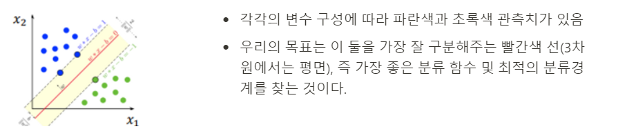
분류경계면을 찾을 때 Generalization(일반화)가 잘 이뤄지는지, 즉 다시 말해 Validation error가 최소인지를 확인해봐야 한다.
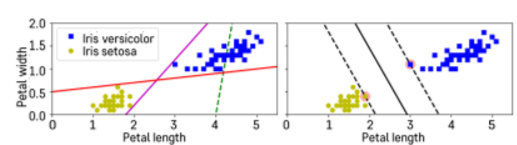
- (오른쪽그림)따라서 실선으로 된 분류경계선에 평행한 점선으로 된 가상 분류경계선을 고려하며, 이때 두 가상 분류 경계선 사이의 거리를 margin이라고 한다.
- 이 떄 가상 분류 경계선은 각각의 클래스를 넘어갈수 없는 것이 가정이다.
- SVM은 두 클래스 사이의 가장 넓이가 큰 분류 경계선을 찾았을 때 가장 optimal하며, 따라서 이를 Large margin classification이라고도한다.
- Support Vector라고 하는 것은 각각의 클래스에서 분류 경계선을 지지하는 관측치들이다.
- 이러한 Support vector들에 의해 최종적인 분류 경계선이 결정되기에 중요하다.
SVM의 주의할 점은 아래와 같다.
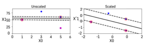
- SVM은 스케일에 민감하기 때문에 변수들 간의 스케일을 잘 맞춰주는 것이 중요하다.
- 관측치들의 스케일을 표준화를 한 다음 분류를 해준다면 더 좋은 성능을 보인다.
- sklearn의 StandardScaler이용
1-2. Hard Margin vs Soft Margin
💡 Hard Margin: 두 클래스가 하나의 선으로 완벽하게 나눠지는 경우에만 적용 가능함
- 분류경계선 안쪽으로 관측치들이 넘어올수 없도록 함
- 하지만 이를 실제로 적용할 수 있는 경우는 극히 드물다. 왜냐하면 이는 두 클래스가 완벽하게 나눠져야 하는 경우여야 하기 때문이다.
💡 Soft Margin: 일부 샘플들이 분류 경계선의 분류 결과에 반하는 경우를 일정 수준 허용하는 방법
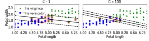
- 이는 SVM의 C 페널티 파라미터로 조정한다.
- C가 작으면 패널티가 낮은것이다. 그래서 왼쪽 그림을 보면 margin이 크다. 하지만 초록색 관측치들이 꽤나 분류 경계선을 넘어가고 있다. 따라서 C가 작으면 margin은 커지지만 오차도 커지는 단점이 있다.
- C가 크며 패널티가 높은 것이다. 오른쪽 그림을 보면 margin은 좁아지지만 training error는 줄어들 수 있다.
- 따라서 margin과 training error 사이의 trade-off가 있음을 알 수 있다.
scaler = StandardScaler()
svm_clf1 = LinearSVC(C=1, loss="hinge", random_state=42)
svm_clf2 = LinearSVC(C=100, loss="hinge", random_state=42)

scaled_svm_clf1 = Pipeline([
        ("scaler", scaler),
        ("linear_svc", svm_clf1),
    ])
scaled_svm_clf2 = Pipeline([
        ("scaler", scaler),
        ("linear_svc", svm_clf2),
    ])

scaled_svm_clf1.fit(X, y)
scaled_svm_clf2.fit(X, y)
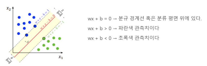
1-3. SVM Prediction
- Classifier: 가상의 분류 경계선 혹은 분류 평면이 도출됨
1-4. Nonlinear SVM Classification
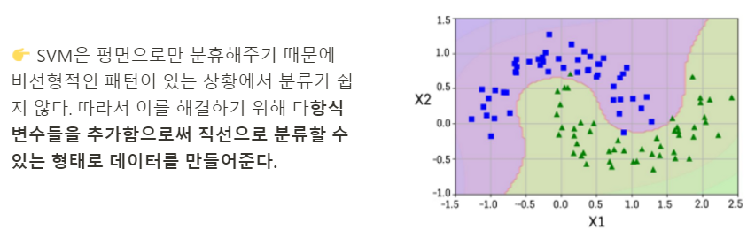
📍 Polynominal Kernel: 다항식의 차수를 조절할 수 있는 효율적인 계산 방법
- 한정된 차원을 가정하고 적용을 하는 것
- 하이퍼파라미터: degree를 조정함
📍 Guassian RBF Kernel: 무한대 차수를 갖는 다항식으로 차원을 확장시키는 효과
- 하이퍼파라미터: gamma(고차항 차수에 대한 가중 정도)
- 커널의 복잡도를 조절하는 파라미터라고 볼 수 있음
👉 C 페널티와 더불어 함께 써준다면 좋은 성능을 낼 수 있다.
2️⃣ SVM Regression
2-1. SVM Regression
- 선형 회귀식을 중심으로 이와 평행한 오차 한계선을 가정하고, 오차 한계선 너비가 최대가 되면서 오차 한계선을 넘어가는 관측치들에 페널티를 부여하는 방식으로 선형 회귀식을 추정한다.
- SVM Classification 모델과 같이 다항식 변수항을 추가하는 개념을 도입함으로써 비선형적인 회귀모형을 적합할 수 있음.
3️⃣ 실습
from sklearn.svm import SVC # SVM Classifier
from sklearn import datasets

# iris데이터
iris = datasets.load_iris()
X = iris["data"][:, (2, 3)]  # petal length, petal width
y = iris["target"]

# 클래스구분
setosa_or_versicolor = (y == 0) | (y == 1)
X = X[setosa_or_versicolor]
y = y[setosa_or_versicolor]

# SVM Classifier model
# kernel="linear": 특별한 패턴을 고려하지 않고 linear한 classification을 만들겠다
# C=float("inf"): hard margins classifier를 학습하고자 한다.
svm_clf = SVC(kernel="linear", C=float("inf"))
svm_clf.fit(X, y)
# Non-linear clafssification
#  **Polynominal Kernel로 그릴 수 있음
from sklearn.svm import SVC

poly_kernel_svm_clf = Pipeline([
        ("scaler", StandardScaler()),
        ("svm_clf", SVC(kernel="poly", degree=3, coef0=1, C=5))
    ])
poly100_kernel_svm_clf = Pipeline([
        ("scaler", StandardScaler()),
        ("svm_clf", SVC(kernel="poly", degree=10, coef0=100, C=5))
    ])

fig, axes = plt.subplots(ncols=2, figsize=(10.5, 4), sharey=True)

plt.sca(axes[0])
plot_predictions(poly_kernel_svm_clf, [-1.5, 2.45, -1, 1.5])
plot_dataset(X, y, [-1.5, 2.4, -1, 1.5])
plt.title(r"$d=3, r=1, C=5$", fontsize=18)

plt.sca(axes[1])
plot_predictions(poly100_kernel_svm_clf, [-1.5, 2.45, -1, 1.5])
plot_dataset(X, y, [-1.5, 2.4, -1, 1.5])
plt.title(r"$d=10, r=100, C=5$", fontsize=18)
plt.ylabel("")

save_fig("moons_kernelized_polynomial_svc_plot")
plt.show()**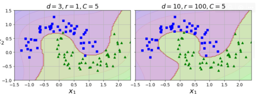
# regression
from sklearn.svm import LinearSVR

svm_reg = LinearSVR(epsilon=1.5, random_state=42)
svm_reg.fit(X, y)
'멋사 AISCOOL 7기 Python > INPUT' 카테고리의 다른 글
| [머신러닝] Ensemble, Bagging, Boosting (0) | 2022.11.24 |
|---|---|
| [KMOOC-실습으로배우는머신러닝] 7.Ensemble Learning (0) | 2022.11.22 |
| [KMOOC-실습으로배우는머신러닝]4. Machine Learning with Optimization: Gradient Descent, Learning rate, Stochastic Gradient Descent, Momentum (0) | 2022.11.22 |
| [KMOOC-실습으로배우는머신러닝]2. Machine Learning Pipeline (0) | 2022.11.21 |
| [KMOOC-실습으로배우는머신러닝] 1. Introduction to Machine Learning (0) | 2022.11.21 |


